It is often possible to write down the equations which describe a physical system, but for which solutions cannot be derived analytically (i.e. the equations are too difficult or impossible to solve directly). In many cases, the only way to solve a specific problem will be using numerical (i.e. computer based) methods. We will look here at the particular case of numerical solutions to 2nd order partial differential equations.
We have an equation involving 2nd partial differentials, such as
| (1) |
which is the equation for a simple harmonic oscillator (e.g. a mass on a spring for which the restorative force is proportional to the extension of the spring).
We require a solution for position and velocity as functions of time, t, i.e. x=x(t) and v=v(t).
We can start by noting that over a short time, Dt, the position of the particle changes by a small amount dx, where
| (2) |
and the velocity of the particle v = dx/dt by a small amount dv where
| (3) |
If we have some initial conditions for x and v, then we can compute what x and v will be a small time later, Dt. If we continue (``iterate'') this step-wise process, the solutions for x(t) and v(t) can be built up from the initial values.
A concrete example in the case of simple harmonic motion:
| (4) |
where we can construct solutions for xn+1 and vn+1, based on the solution at an earlier time, xn and vn, after a time step Dt
| (5) |
| (6) |
At this point we haven't done much until we carry out a splendid trick of using the differential equation to substitute for d2x/dt2:
| (7) |
The solution can now be built up step-wise, starting from x0 = x(0) and v0 = v(0).
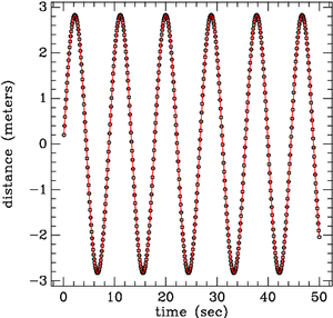
The first fortran program (shm.f) in the Appendix demonstrates this technique: starting from an initial position x0=0 with an initial velocity v=v0 at time t=0, it solves the equation of simple harmonic motion, giving the position and velocity for 500 time steps of 0.1 seconds each.
This is a system for which the analytical solution is known :
| (8) |
Figure 4.1 shows the results of the program. The numerical solution for the position is plotted as a function of time (circles). The analytical solution is shown by the line, and is a very close match.

In the last lecture, we have solved for the linear and constant density models of a star. These models are the simplest one can construct, but are not very physical.
This week we examine a physically motivated model, in which a simple form for the pressure as a function of the density is adopted
| (9) |
where K and g are constants.
It is usual to express g in terms of the polytropic index n, where
| (10) |
Starting from the equation of Hydrostatic equilibrium,
| (11) |
and the mass equation,
| (12) |
one can eliminate the mass by differentiation with respect to r to obtain
| (13) |
|
Problem 4.2 Verify the relation above. Substitute P = K rg and show that
|
We now have a second order differential equation in r as a function of the radius r.
We introduce a dimensionless radius, x, where r = a x, and a is a constant scale factor, and a dimensionless density function f which is related to the stellar central density, rc by r = rc fn. In these new dimensionless variables (x and f), the pressure equation becomes (remembering that g = 1 + 1/n)
| (15) |
|
Problem 4.3 Substituting for P into the equation derived in Problem 4.2 above, show that
|
An appropriate choice for a is
| (17) |
Using this as our definition of a, we obtain the Lane-Emden Equation
| (18) |
The boundary conditions for this equation come from the central density
| (19) |
and from the equation of Hydrostatic Equilibrium, we know that
| (20) |
and so
| (21) |
Three analytical solutions to the Lane-Emden equation are known, for n = 0, 1 and 5.
|
Problem 4.4 Show that the following are solutions to the L-E equation of index n
n = 0, f(x) = 1 - [(x2)/6]
n = 1, f(x) = [(sin(x))/(x)]
n = 5, f(x) = [ 1/(Ö{1 + [(x2)/3]})]
|
Further solutions must be obtained numerically, i.e. by computer, and we will look at this topic next.
Solving the Lane-Emden equation is only slightly more complicated than the simple harmonic motion example above. We start by expressing the equation in the form
| (22) |
|
Problem 4.5 Verify this form of the Lane-Emden equation.
|
We are interested in solving for the dimensionless density, f as a function of the dimensionless radius x.
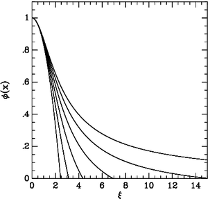
The second program in the Appendix (laneem.f) solves the L-E equation. It uses the same method of stepping forward from initial conditions, in this case f(0) = 1 and df/dx = 0.

|
Problem 4.6 Use this program to solve the L-E equation for a range of indices, n, (e.g. 0, 0.5, 1, 1.5, 2.0, ...). For each solution, determine where f = 0 to an accuracy of two decimal places (i.e. determine the "root" of the equation, and the radius of the surface of the star). For indices, n, of the equation for which an exact, analytical solution is known, use gnuplot to plot and compare the numerical and analytical solutions.
|
FORTRAN is a very widely used programming language, particularly by scientists and engineers. The name is derived from FORmula TRANslation. It began development in the 1950's and has been actively developed to meet the needs of new generations of programers to the present day. It's wide use is because of its simplicity, portability and reliability. Many types of problems have already been solved using Fortran, so that one can very often find existing Fortran to solve a particular problem.
What follows is a very quick guide to Fortran. The concepts introduced below apply to virtually any programming language (BASIC, C, C++, Pascal, Mathematica, Fortran, Java etc.)
From the course website you can get a public domain Fortran compiler, called bcf, which was written by A. Koestl. It is used to translate the Fortran examples below into executable programs on a PC running DOS.
Start by getting all the files and putting them into a subdirectory, called (e.g.) bcf. To run the program, start a DOS window, go to the subdirectory (cd bcf) and first run the small program
c:\bcf> bcrtsy
the system will then be ready to run fortran.
Here is the first demonstration program, called hello.f:
       program hello
       write(6,*) 'Hello, world!'
       end
Note that there are 7 spaces at the start of each line before the command. Without these spaces the program won't work! The reason for these spaces will be shown later.
to compile this program, do
bcf hello.f
and to link the result do
bcl hello lib.b
this will create a file called hello.exe, which you can run:
hello
and the result will be a line printed on the screen
Hello, world!
Note that the error messages when this compiler operates are in German, so if you need translations they are stored in the file english.txt (along with other info which may or may not be useful at this stage!).
For an easy to follow user's guide to BCF fortran, see http://personal.cfw.com/~terry2/tutorial/.
Now let's do something more interesting. Here's a program (linear.f) to compute the central physical values for the linear solar model above.
        program linear

* calculates the temperature, pressure and mass as a
* function of normalised radius (r=1 is at stellar surface)
* for a linear stellar model of the Sun

        real m,Msun,mu,mp,k          ! all these variables are real numbers

* open a file for the results of the calculation

        open(20,file='linear.dat',status='unknown')

        G =  6.67259E-8        ! Gravitational constant in cm^3 / gram sec^2
        Msun = 1.99E+33               ! solar mass in grams
        Rsun = 69600000000.           ! solar radius in cm
        pi = 3.14159265
        mu = 1.0*0.90/2.0 + 4.0*0.10/3.0    ! mean molecular weight, assuming
                                      ! 90\% Hydrogen and 10\% Helium
        mp = 1.672631E-24             ! Mass of a proton in grams
        k =  1.380658E-16             ! Boltzmann constant in erg/Kelvin

* compute central density, pressure and temperature

        rho0 = 3.0*Msun/(pi*Rsun**3)                 ! central density
        P0 = (5.0*G*Msun**2)/(4.0*pi*Rsun**4)        ! central pressure
        T0 = (5.0*pi*G*mu*mp*rho0*Rsun**2)/(36.0*k)  ! central temp

        write(6,*) 'Solar Mass= ',Msun
        write(6,*) 'Solar Radius = ',Rsun
        write(6,*) 'Central pressure = ',P0
        write(6,*) 'Central temperature = ',T0
        write(6,*) 'Central density = ',rho0
        write(6,*) 'Mean molecular weight = ',mu

        end
As before, to compile this program, do
bcf linear.f
and to link the result do
bcl linear lib.b
To run the program:
linear
and the results will be printed to the screen
 Solar Mass=   1.99E+33
 Solar Radius =   6.96E+10
 Central pressure =   4.5E+15
 Central temperature =   5.6E6
 Central density =   5.6
 Mean molecular weight = 0.58
The fortran program linear.f above does much the same as the Gnuplot program from the previous lecture, except that it doesn't yet determine the temperature, density and pressure profiles for the star, just the central values. To add this capability to the program, we need the concept of the ``loop''. A loop controls the number of times that a specific action should be repeated.
       program loop_demo
* demonstrates the use of a loop in fortran
* to calculate (2x)**2 for x = 2, 4, 6, ..., 20

       do i = 1, 10
          x = 2.0*i
          write(6,*) x,x**2
       end do

       end
The output of this program is
  2.  4.
  4.  16.
  6.  36.
  8.  64.
  10.  100.
  12.  144.
  14.  196.
  16.  256.
  18.  324.
  20.  400.
The loop is controlled by the variable i, which is an integer and takes values from 1 to 10 in steps of 1.
A final demonstration program (tempconv.f) computes a table of Celsius to Fahrenheit conversions and vice versa:
      program fortrandemo

c program to demonstrate basic usage of fortran
c lines starting with a 'c' are called 'comments'
c and are ignored by the computer

c declare (define) the following 'variables' in the program
      real c,f,c1,f1
      integer i

c compute celsius to fahrenheit (and vice versa) tables and
c write out in a nice fomat
c first write out the table header

      write(6,*) '                                       '
      write(6,*) ' +------------------------------------+'
      write(6,*) ' |    Temperature Conversion Table    |'
      write(6,*) ' |------------------------------------|'
      write(6,*) ' |     C       F   |      F      C    |'

c starting temperatures in celsius and fahrenheit
      c = -30.0
      f1 = -25.0
c now a loop to compute C->F and F->C in steps of 5 degrees in C
c and steps of 10 degrees in F

      do 10 i = 1, 15
         f = c*(9.0/5.0) + 32.0
         c1 = (f1-32.0)*(5.0/9.0)
         write(6,'(a3,2f8.1,a2,2f8.1,a)') '  |',c,f,' |',f1,c1,'  |'
         c = c + 5.0
         f1 = f1 + 10.0
 10   continue

c finished the computations, write the end of the table

      write(6,*) ' +------------------------------------+'
      write(6,*) '                                       '

c that's all folks!

      end
Here is what the program outputs:
  +------------------------------------+
  |    Temperature Conversion Table    |
  |------------------------------------|
  |     C       F   |      F      C    |
  |   -30.0   -22.0 |   -25.0   -31.7  |
  |   -25.0   -13.0 |   -15.0   -26.1  |
  |   -20.0    -4.0 |    -5.0   -20.6  |
  |   -15.0     5.0 |     5.0   -15.0  |
  |   -10.0    14.0 |    15.0    -9.4  |
  |    -5.0    23.0 |    25.0    -3.9  |
  |     0.0    32.0 |    35.0     1.7  |
  |     5.0    41.0 |    45.0     7.2  |
  |    10.0    50.0 |    55.0    12.8  |
  |    15.0    59.0 |    65.0    18.3  |
  |    20.0    68.0 |    75.0    23.9  |
  |    25.0    77.0 |    85.0    29.4  |
  |    30.0    86.0 |    95.0    35.0  |
  |    35.0    95.0 |   105.0    40.6  |
  |    40.0   104.0 |   115.0    46.1  |
  +------------------------------------+
All the programs above demonstrate the basic concepts of computation with Fortran, but are mostly things you could do simply with a calculator or Gnuplot. The following examples demonstrate where a language like Fortran has its real power - solving an equation numerically which cannot be solved analytically. We start with an example (shm.f) of the equations for Simple Harmonic Motion (SHM) where the analytical solution is known, so that we can compare to the numerical solution.
        program shm

c**************************************************************
c* program to solve numerically a system executing simple     *
c* harmonic motion (shm)                                      *
c*                                                            *
c* the equation of motion is                                  *
c* d^2x/dt^2 = - K * x                                        *
c*                                                            *
c* initial conditions are x = x0 and v = dx/dt = v0           *
c*                                                            *
c*                                                            *
c* and the analytical solution is                             *
c* x = v0/sqrt(k) * sin (sqrt(k)*t)                           *
c*                                                            *
c* results stored in the file shm.dat                         *
c*                                                            *
c* CF. Oct 1999.                                              *
c**************************************************************

        real x, v, v0, t, K, exact

* K is the force constant (units = sec**-2)

        K = 0.5

* variables and units are
* position : x (meters)
* velocity : v (meters/second)
* time : t (seconds)

* specify initial values

        x = 0.0
        v0 = 2.0
        v = v0
        t = 0.0

* "time step" is in seconds
* the smaller the time step the more accurate the calculation
* and the longer it takes!

        dt = 0.1

* open the file for output of results
        open(20,file='shm.dat',status='new')

* now the MAIN program loop
        do 100 i = 1, 500

* calculate the change in velocity
          v = v - K*x*dt

* calculate the change in the position
          x = x + v*dt

* increment the time
          t = t + dt

* compute exact solution to the equation
          exact = v0/sqrt(K)*sin(sqrt(K)*t)

* write out the results
          write(20,*) t,x,v,exact

100     continue

        end
The program stops when f becomes negative. At this point, x is the radius of the star, which we have denoted xR in the lecture.
Note well that for n ł 5, the solution never becomes negative, so the program will never stop!
        program laneem

c**************************************************************
c* program to solve the Lane-Emden equation numerically       *
c*                                                            *
c* the equation to solve is                                   *
c* d^2x/dt^2 = - ((2/t)*(dx/dt) + x**n)                       *
c*                                                            *
c* where x is the dimensionless density function (psi)        *
c* and t is the dimensionless length (xi)                     *
c* initial conditions are      x = 1 and dx/dt = 0            *
c*                                                            *
c* and the power index is n.                                  *
c* analytical solutions are known for n=0, 1, 5.              *
c*                                                            *
c* CF. Oct 1999.                                              *
c**************************************************************

        real x, dxdt, n, dt, xlast, dxdtlast
        character*50 name

* index n of the polytrope

        write(6,*) 'Enter n, the polytrope index '
        read(5,*) n

        if (n.ge.5) then
          write(6,*) 'n is too big, star radius is infinite'
          stop
        end if

        write(6,*) 'Enter name of results file'
        read(5,*) name

* open the file for output of results

        open(20,file=name,status='new')

* variables are
* dimensionless length : t
* dimensionless density function : x

* specify initial values

        x    = 1.0
        dxdt = 0.0
        t    = 0.0001

* "radius step" is in length variable, t
* the smaller the step the more accurate the calculation
* and the longer it takes!

        dt = 0.001

* now the MAIN program loop

        do 100 i = 1, 10000

* calculate the next dxdt
          dxdt = dxdt - ( 2.0*dxdt/t + x**n )*dt

* calculate the next x
          x = x + dxdt*dt

* increment the dimensionless radius (move outward in the star)
          t = t + dt

* write out the results

          write(20,*) t,x,dxdt

* check if the solution has become negative yet
          if (x.lt.0.0) goto 999

100     continue

999     continue

        end