Lecture 3 : Modeling Stars

1  Basic concepts

A star is a self gravitating ball of gas. There are two basic forces at work, on one hand gravity, which is attempting to make the star collapse inward on itself, and on the other hand there is the generation of energy and pressure from within the star, which holds the star up.

1.1  Energy from the Solar Surface

The sun radiates 1.374 ×10⁶ ergs/sec/cm² at the surface of the Earth, or about 1.4 kW per square meter, a quantity called the solar constant. The Sun's mean distance from us is 1.496 ×10¹³ cm (or 1 astronomical unit = 1 A.U.) and hence its luminosity is

LO = 3.86 ×1033 erg/sec.

(1)

2  Stellar time scales

2.1  Free fall time-scale

If there were no outward force holding a star up against gravity, how long would it take to collapse? This quantity is called the ``free-fall'' time scale, t_ff.

We allow a test particle to fall from the surface of the star of radius R and mass M. Its distance from the star center is given by r. Its acceleration is then

d2r dt2 = -  GM r2

(2)

where G is the gravitational constant.

Integrating this equation, and using the boundary condition r = R at t = 0, leads to the free-fall time

tff =  1 2 (  R3 GM )1/2

(3)

Using the mass and radius of the Sun,

MO = 1.99 ×1030 kg,  and   RO = 6.96 ×1010cm

(4)

we derive the Solar free fall time t_ff = 27 minutes.

This is a very short time! The Sun would collapse on this time-scale were it not for the pressure support due to the outward flow of generated energy.

2.2  Kelvin-Helmholtz time-scale

One idea proposed in the 19th century as the source of the Sun's energy is gravitational contraction. If a massive body gets smaller, it releases gravitational potential energy, in this case in the form of heat.

The gravitational potential energy is given by the integral over

W = -  G m m¢ r

(6)

for masses m and m¢ separated by a distance r.

For a spherical body, such as a star, one finds (to within a small constant)

W =  M2 G R .

(7)

For the Sun, this is W_O = 4 ×10⁴⁸ erg.

Suppose now that the Sun is collapsing slowly in order to generate its luminosity. How long would it be able to shine? This time scale is called the Kelvin-Helmholtz time-scale, t_KH.

The solar luminosity is L_O = 3.86 ×10³³ erg/sec, hence the Sun can shine at this rate by converting potential energy for

tKH =  4 ×1048 erg 4 ×1033 erg/sec = 1015 sec = 30 Myr.

(8)

This is quite a long time, and in the middle of the 19th century, when it was first derived, it was considered to be the best estimate for the age of the Sun. Late in the 19th century and early in the 20th, the age of the Earth became much better understood than the age of the Sun, with geological evidence and radioactivity indicating that it is billions of years old. There was quite a conflict between the old and young age scales until the realisation that there is a third source of energy which is capable of sustaining the stars, nuclear energy.

2.3  Einstein time-scale

The amount of energy in the Sun in its rest mass, M_O, is given by

E = MO c2 = 2 ×1054 ergs.

(9)

The Einstein time scale, t_E, is then

tE =  2 ×1054 erg 4 ×1033 erg/sec = 5 ×1020 sec = 1013 years.

(10)

Here we assume that all the rest mass energy is converted into radiation - i.e. the Sun radiates and finally disappears when it is finished burning!

Detailed analysis reveals that the Sun will be about 0.1% efficient in converting its mass into radiant energy, and the lifetime for a star like the Sun is therefore reduced by this factor to circa 10¹⁰ years, or about the present age of the Universe.

3  Hydrostatic Equilibrium

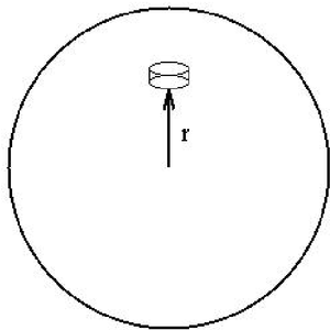
Consider a small mass element at a distance r from the center of a spherical body, with density r, area A and thickness dr (see Figure 3.1). The gravitational force inward on the mass element is given by

FG = G  M(r) rA dr r2

(11)

where M(r) is the mass of the body inside radius r.

The pressure force outward on the mass element is related to the difference between the pressure on the upper surface of the mass element and the lower surface. We denote this pressure difference dP.

FP = - A dP.

(12)

For a star in mechanical equilibrium, these forces balance, so that

FP + FG = 0

(13)

We can use this equation to derive first order estimates of the temperature and pressure at the center of the Sun.

3.1  Solar central pressure

To first order, we can consider dP/dr as the pressure difference between the edge and the center of the sun. From Eqn 3.14, we have

P(r=0) - P(r=RO) 0-RO = - GMO r/RO2

(15)

using the mean density of the sun, r = M_O/((4 p/3)R_O³), and assuming that the central pressure is much greater than the surface pressure, we get

Pcentral =  3 4p G M2O/RO4 = 5 ×1015 dyncm-2

(16)

or about 5 ×10⁹ atmospheres. Obviously the above approximation was very rough, and a careful analysis shows that it is about two orders of magnitude too small. However, it is not a too bad first approximation.

3.2  Solar central temperature

We now have an estimate of the central pressure, and assuming that the material at the center is a still a gas, we can relate this pressure to the temperature, T, and the Boltzmann constant k via the equation of state for an ideal gas:

P = NkT

(17)

where N is the number density of particles.

A detailed analysis shows that the central solar temperature is about 15×10⁶ K, so this simple estimate is not too bad.

4  Structure of a star in equilibrium

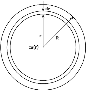
Consider the equation of Hydrostatic equilibrium in terms of the mean density r of a spherical shell within a spherically symmetric star.

dP dr = -  Gm(r)r(r) r2

(18)

Here P(r) is the pressure as a function of radius, r; m(r) is the mass inside radius r, and G is the gravitational constant (see Figure 3.2). The mass of the shell dm, is given by its area, thickness dr and density r

dm = 4 prr2 dr

(19)

The two equations above can be combined to give

dP dm = -  Gm 4 pr(m)4

(20)

where the radius is now treated as a function of the interior mass, r = r(m). This equation can be integrated to derive a result for the maximum central density of the star, by considering the quantity P¢

P¢ = P +  m2G 8 pr4

(21)

The problem above shows that [(dP¢)/dr] is always negative going outward from the center of the star, so it follows that P¢ always decreases going outward. At the center of the star, the second term in the quantity P¢ approaches 0, and hence P¢ approaches the central pressure P_cen. It follows that

Pcen >  M2G 8 pR4

(22)

This sets a lower limit to the central pressure in a star.

Figure 2: Hydrostatic equilibrium

5  Simple stellar models

We cannot integrate the equation of hydrostatic equilibrium to derive the behaviour of temperature, density, pressure etc without further assumptions about the physics of energy production and the manner in which it is transfered to the surface. However, several instructive ``toy models'' can be developed which give an idea of the kind of behaviour we can expect. We will look at two such models, the linear stellar model and (later) the so-called polytropes.

In the first of these models the density of the star takes an arbitrarily assumed form, which decreases linearly from the center to the surface.

r = rcen  (r - R) R

(23)

In the second model a simple form for the pressure as a function of the density is adopted

P = K rg

(24)

where K and g are constants.

5.1  Linear stellar model

Assuming that the density in a star varies linearly with radius as

r = rcen æ è 1 -  r R ö ø

(25)

we use the equation of hydrostatic equilibrium to derive

dP dr = -  Gm(r)rcen r2 (1 -  r R )

(26)

From Eqn 3.19 the mass varies with the radius as

dm = 4 prcen(1-  r R ) r2 dr.

(27)

Integrating we get

m(r) = pr3 rcen (  4 3 -  r R )

(28)

We can normalise the equation to the total mass, M, by noting that at r=R,

M = pR3 rcen (  4 3 - 1) =  pR3 rcen 3 .

(29)

Substituting for r_cen, we derive

m(r) = M (  r R )3 (4 -  3r R )

(30)

Inserting this result into the equation of hydrostatic equilibrium (Eqn 3.26), we derive

dP dr = -pGrcen2r(  4 3 -  r R )(1-  r R )

(31)

Substituting for the central density r_cen (from Eqn 3.29), we derive

Pcen =  5G 4p  M2 R4

(33)

One can derive the temperature profile in the star by substituting the equation of state for an ideal gas, T = mm_H P/rk, where m_H is the proton mass and k is the Boltzmann constant, and m is the mean molecular weight, (N.B. this assumes that the only pressure term is due to the gas pressure - i.e. the photon pressure is ignored).

5.2  Constant density stellar model

A specific instance of the linear model is one in which the density is constant - i.e. there is no gradient in the density

r = rcen

(35)

We can use this model to rederive our results in the previous section for the central pressure and central temperature. We have:

dP dr = -  Gm(r) r2 r(r)

(36)

and

m(r) =  4 pr3 3 rcen

(37)

substituting for m(r) into Eqn 3.36 and integrating (using the boundary condition that P=0 at the surface of the star r=R) we obtain as a constant of the integration the central pressure

Pcen =  2 p 3 G rcen2 R2

(38)

and since the density is constant, the mean density is the same as the central density

rcen =  3 M 4 pR3

(39)

and so we derive a central pressure of

Pcen =  3 G M2 8 pR4 .

(40)

The pressure as a function of the radius is given by

P(r) =  3 G M2 8 pR6 (R2-r2).

(41)

6  Gnuplot

In class you'll get a floppy disk containing the public domain program GNUPLOT, published by the Gnu Foundation.

A good site for help with gnuplot is at
http://www.cs.uni.edu/Help/gnuplot/.

You can get the windows version of the program from
http://www.astro.utu.fi/~cflynn/Stars/gnuplot3_7cyg.zip.

Here is a quick guide to doing some basic things. Start gnuplot by clicking on the icon or typing gnuplot.

To plot out a simple function:

gnuplot> plot sin(x) 

to plot with some parameters set:

gnuplot> plot f(x) = sin(x*a), a = 0.2, f(x)

to plot with x and y axis limits

gnuplot> plot [t=1:10] [-pi:pi*2] tan(t) 

set range of X-axis

gnuplot> set xrange [1:10] 

set range of Y-axis

gnuplot> set yrange [-pi:pi]

plot out a parabola

gnuplot> set xrange[-10:10]
gnuplot> f(x) = x**2
gnuplot> plot f(x)

plot data from a file

gnuplot> plot 'fig5.dat'

define a 2-D function

gnuplot> f(x,y) = x**2+y**2

plot a 2-D function

gnuplot> splot f(x,y)

same with ranges set

gnuplot> splot [x=-5:5] [y=-5:5] [0:200] f(x,y)

define X-axis label

gnuplot> set xlabel "radius [r/R]"

define Y-axis label

gnuplot> set xlabel "temperature [T/Tc]"

Example input file (e.g. ``linear.gp''):

t(x) = 1.0 + x - (19.0/5.0)*x**2 + (9.0/5.0)*x**3
m(x) = 4.0*x**3 - 3.0*x**4

read commands from this file

gnuplot> load "linear.gp"

plot several functions

gnuplot> plot t(x),m(x)

7  Linear Solar Model

Continuing from the last section, where we derived basic results for the linear stellar model, we will look this week at a practical example of programming to solve the model for the specific case of the Sun.

We would like to determine the pressure, P(r), and temperature, T(r) profiles for the Sun in this model as a function of radius, r:

P(r) =  5pG 36 rcen2 R2 (1 -  24r2 5R2 +  28r3 5R3 -  9r4 5R4 )

(42)

T(r) =  5pG mmp 36 k rcen R2 (1 +  r R -  19r2 5R2 +  9r3 5R3 ).

(43)

From these expressions it is easy to see that the central pressure and central temperature (at r=0) are given by

P0 =  5pG 36 rcen2 R2

(44)

and

T0 =  5pG mmp 36 k rcen R2.

(45)

The density r(r) falls linearly with radius and is given by

r = rcen  (R - r) R .

(46)

where the central density can be found from (Eqn 3.29)

M =  pR3 rcen 3 .

(47)

i.e. for the Sun

rcen =  3 MO pRO3 .

(48)

Here is a listing of the Gnuplot commands needed to plot the temperature as a function of radius in the Sun. The physical quantities needed for a linear model of the Sun are listed in Table 3.1.

# first, define the values of constants

gnuplot>  G =  6.67259E-8      
gnuplot>  Msun = 1.99E+33  
gnuplot>  Rsun = 6.96E10  
gnuplot>  mu = 0.6
gnuplot>  mp = 1.672631E-24
gnuplot>  k =  1.380658E-16 

# now compute central values of P, T and rho

gnuplot>  P0 = (5.0*G*Msun**2)/(4.0*pi*Rsun**4) 
gnuplot>  rho0 = 3.0*Msun/(pi*Rsun**3)  
gnuplot>  T0 = (5.0*pi*G*mu*mp*rho0*Rsun**2)/(36.0*k)

# Print out the results

gnuplot>  print "Central Pressure = ", P0
gnuplot>  print "Central Temperature = ", T0 
gnuplot>  print "Central Density = ",rho0

# Plot the temperature profile, T

gnuplot>  t(x) = T0*(1.0 + x -(19.0/5.0)*x**2 + (9.0/5.0)*x**3) 
gnuplot>  plot [0:1] t(x) 

References

[]

R. Bowers and T. Deeming in Astrophysics I, Stars, 1984, Jones and Bartlett Publishers

[]

W. Press, Astrophysics Lecture Notes, Chapter 5. http://cfata2.harvard.edu/whp/ay45top.html