In the previous lecture we developed some simple spherical potential-density pairs which can be used to model the mass distribution and the stellar orbits in galaxies. These were for a point mass, a uniform or homogeneous sphere and for the isothermal sphere. The following table summarises results for each configuration, adopting mass M and scale length a (note that the isothermal sphere is described in terms of central density since its mass diverges at large r):
| Φ(r) | ρ(r) | V2circ | |
| Point mass | −GM/r | N/A | GM/r |
| Uniform sphere | −3GM (a2−r2/3)/2a3 | 3M/4πa3 | GMr2/2a3 for r < a |
| −GM/r | 0 | GM/r for r ≥ a | |
| Isothermal sphere | 4πGρ(0)a2 ln(r/a) | ρ(0) (r/a)−2 | 4πGρ(0)a2 |
Three more functions often used in the literature are the Plummer, Hernquist and Jaffe spheres:
Φ(r)
ρ(r)
V2circ
Plummer
−GM(r2+a2)−1/2
(3M/4πa3)(1+(r/a)2)−5/2
GMr2(r2+a2)−3/2
Hernquist
−GM/(r+a)
(M/2πa3) a4/(r(r+a)3)
GMr(r+a)−2
Jaffe
GM/a ln(r/(r+a))
(M/4πa3) a4/(r2(r+a)2)
GM/(r+a)
| Exercise #1: Starting from the potential Φ in each case, verify the derived forms for density and circular velocity in the tables. |
The density distributions for some of these distributions are shown below. Each one has been normalised to ρ=1 at r = 1.
The Plummer (MNRAS, 71, 460, (1911)) density profile has a finite-density core and falls off as r-5 at large radii; this is a steeper fall-off than is generally seen in galaxies.
The Hernquist (Astrophysical Journal, 356, 359, (1990)) and Jaffe (MNRAS, 202, 995, (1983)) models, on the other hand, both decline like r−4 at large radii. The Hernquist model has a gentle power-law cusp (a steepening of the profile in the core). The Jaffe model has an even steeper cusp.
The following plots show an image of the density distribution of each model, along with the generating potential and the circular velocity as a function of distance from the center.
Plummer model
| Exercise #2: Show that the falloff with density at large radius r goes like r−5 for the Plummer sphere, and like r−4 for the Hernquist and Jaffe models. How does the density fall off at large radius for the isothermal sphere? |
We start from a Plummer sphere, with mass M and scale length b.
Now consider a cylindrical
coordinate system (R, z) where R is the radius in the plane and z is the
height above the plane:
Φ(r)
ρ(r)
V2circ
Plummer
−GM(r2+b2)−1/2
(3M/4πb3)(1+(r/b)2)−5/2
GMr2(r2+b2)−3/2
We introduce the following potential as a modification of the Plummer form above, and which is due to Miyamoto and Nagai (Pub. Astron. Soc. Japan., 27, 533, (1975)).
| Φ(r) | ρ(r) | |
| Miyamoto-Nagai | −GM | Mb2 [aR2 + (a + 3(z2+b2)1/2)(a + (z2+b2)1/2)2] |
| |
|
|
| [R2+(a+ (z2+b2)1/2)2]1/2 | 4π [R2 + (a + (z2+b2)1/2)2 ]5/2(z2+b2)3/2 |
This reduces to the Plummer potential for a = 0, while for b = 0 it
reduces to a potential generated by an infinitely thin disc (Kuzmin
1956) -- in other words, the potential can be used to generate
anything from an infinitely thin disk to a spherical system, by
varying the parameters a and b.
Some examples of the density in the plane of cross-section (R, z)
are shown below for different values of b/a (from left to right, they
are a/b=0.1, 0.2 and 1.0).
The Miyamoto-Nagai potentials are clearly very useful for generating simple
disk-like density distributions! That's what we'll do next.
Recall from Lecture 1 that the basic components of the Milky Way are the
visible disk and spheroid, and the invisible dark matter halo.
For the bulge (spheroid) we adopt a Plummer sphere, for the disk we
adopt three Miyamoto-Nagai potentials which are added together in order
to reproduce the scale length of the disk, and for the dark matter halo we
adopt a logarithmic (modified isothermal sphere) potential, which
produces a flat rotation curve at large radius. The model is from Flynn et al
MNRAS, 281, 1027
(1996). It is very typical of models of the Galactic potential, which date
back to
Schmidt (BAN, 13, 15, (1956)) and
Innanen, (Zeitschrift für Astrophysik, Vol. 64, p.158 (1966)). This model
includes a dark halo though, as has been the habit since the dark halos were
discovered in the late 1970s. More on dark halos later!
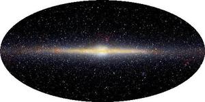
The projected mass
distribution for this model Milky Way is shown below. The main difference
between this model and the actual infrared image is the shape of the bulge ---
it is clearly not round in the real galaxy.
Dirbe (Infrared) Image of the Milky Way. Source http://map.gsfc.nasa.gov/html/milky_way.html
A Galaxy Model
We will now combine three
of the potential-density forms above to produce a model of the matter distribution
and its gravitational potential of the Milky Way.
| Exercise #2: In the IR image, there is more light on one side of the disk than the other --- the Galaxy is not quite symmetric around the center. What could be going in in the inner galaxy which is missing from the model? |
The orbital velocity for circular orbits as a function of distance from the
center of the Milky Way is shown by the black line below. The individual
contributions of each component are marked for the spheroid (green), dark halo
(red) and the disk (blue). Note that the disk and spheroid together account for
most of the rotation cuve within the solar circle (at 8 kpc). The rotation
curve is really only different from that expected from the models of the
visible components (disk+spheroid) in the outer regions of the Milky
Way.
 |
| Exercise #3: look at the total circular velocity (black curve) of the model, and compare it to the circular velocity due to the individual components in the model. The total circular velocity is clearly not computed as a simple sum of the individual components. How is the total velocity being computed? You may need to look back through the definitions of potential Φ and circular velocity. |
 |
| Exercise #4: make an estimate of the expected rotation curve of the model galaxy if you ignore the contribution of the (dark) halo. How does your estimated curve compare to the observed roation curve above? |
 |
The surface density of matter in the disk is shown above as a function of radius. The distribution is close to exponential as is actually observed in most disk galaxies. The scale length of the exponential disk of the Milky Way is difficult to measure, and a good range of estimates exist, lying typically in the range 2.5 to 5 kpc. The scalelength of the model disk here is around 4.1 kpc, at the upper end of the range.
| Exercise #5: from the surface density plot of matter in the disk as a function of radius, make an estimate of the total mass of the disk. You might start out by verifying that the distribution is reasonably fit by an exponential function of scalelength approx 4 kpc. |